


Ever wondered how geo-data works? If you have ever used any of the following on a device or PC – maps for navigation, ride-sharing or food delivery services, then likely you have come across geo-data from the lens of a consumer. But how does geo-data work from the perspective of someone in a data role such as a Data Analyst, Engineer or Scientist? Once it is understood, geo-data becomes a powerful mechanism to answer many location based questions like Which customers sit within a specific delivery radius? What happens if this expands by x distance? Do sales territories overlap?
This article is an explainer on getting started with geo-data and aims to cover:
- Storage: What exactly is geo-data? How is it stored in a database? What does it look like?
- Querying: What functions are available to query and analyse geo-data?
- Visualizing: Mini case study demonstrating each of the above points.
There are two broad types of Geo-data,
- Vector – This is coordinate‑based
- Raster – This is grid and value based
Raster is gridded imagery and often used for satellite photos, elevation models but is out of scope here. This article covers the Vector data type from here on in.
Storage
What exactly is Geo-data?
Geo-data in its simplest form is a set of coordinates. Think of a treasure map drawn containing gridlines. It features:
- Dots marked with an “X” indicating where the treasure is.
- Lines trace the path to get there.
- Shapes outline the objects that can be expected along the way.
This map is a good, basic representation of geo-data in visual form. Behind the visual are a set of numbers that represent coordinates along a 2-dimensional grid. The ‘X’ marks a specific point or set of coordinates on the map, the line marks a series of coordinates specified in an order and the shape is a line that loops back to its starting point.

Figure 1 – Geo-data is simply numbers representing coordinates on a map

Figure 2 – Lat/long coordinates on Earth form the foundation of geo-data
Working with geo-data is very similar to this treasure map. Except the grid lines are located across Earth and the coordinates are widely known as Latitude and Longitude. The 3 common types of Vector geo-data were described earlier and they are Points, Lines and Shapes.
| Geo-data type | Description | Example |
|---|---|---|
| Point | A single set latitude/longitude coordinates. | Location of building |
| Line | Coordinates in a sequence. | River |
| Polygon (shape) | Coordinated in a sequence chained together that covers an area | Delivery radius |
Table 1- Three commonly used types of geo-data
How is geo-data stored in a database?
Now that we have learnt that geo-data is essentially numbers, how is it stored in a database? It’s not stored as plain text or even integer/decimals. Most database engines have geospatial extensions that facilitate the storage and analysis of geo-data. One such database engine is PostgreSQL, an open-source engine with the PostGIS (PostgreSQL Geographic Information System) framework that allows for spatial objects. This means it knows how to read certain objects and interpret them as latitude/longitude coordinates. PostGIS is unique to PostgreSQL but the functions used in this guide are fairly universal across most geospatial equivalent frameworks in other database engines. Across the 3 types of geo-data, they are stored as:
| Geo-data type | Stored in database |
|---|---|
| Point | POINT(151.2093 ‑33.8688) |
| Line | LINESTRING(151.2485 ‑33.1423, 149.1209 ‑35.2809) |
| Polygon (shape) | POLYGON((144.9543 ‑37.8101, 144.9758 ‑37.8090, 144.9843 ‑37.8222, 144.9518 ‑37.8248, 144.9535 ‑37.8650)) |
Table 2 – How geo-data types are stored in a database
In the table above, lat/lon coordinates are specified within some keywords (POINT, LINESTRING, POLYGON). These are type labels and are part of a broader format of WKT (well known text) that informs the database engine the object that is being dealt with. ie, If POINT(lon lat), then WKT is informing the database of a single coordinate, if POLYGON((lon1 lat1, … lonN latN)), then it’s being informed of shape made up of multiple coordinates that enclose an area. Coordinates also require additional configuration and all examples in this article use WGS‑84 (SRID 4326).
Why do decimals matter?
From the examples above, each set of coordinates were rounded off to 4 decimal places. Each extra decimal place makes a significant difference to how ‘precise’ the location is. The following table is an approximation on this:
| Decimals | Approximate precision |
|---|---|
| 2 | ~1km |
| 4 | ~10m |
| 6 | ~10cm |
Table 3 – a couple of decimals can be the difference between a few centimeters and 1km
What does Geo-data look like?
The open source database engine, PostgreSQL, is used in the examples mentioned in this article configured with the PostGIS extension.
The PostGIS extension needs to be installed and created in PostgreSQL as an initial set up step.
-- Enable PostGIS once per database
CREATE EXTENSION IF NOT EXISTS postgis;
The code below is an example of creating a table and inserting geo-data:
DROP TABLE IF EXISTS geo_demo;
CREATE TABLE geo_demo (
    id         SERIAL PRIMARY KEY,
    name       TEXT,
    loc_point  GEOMETRY(POINT,     4326),   -- now geometry
    path_line  GEOMETRY(LINESTRING,4326),
    area_poly  GEOMETRY(POLYGON,   4326)
);

INSERT INTO geo_demo (name, loc_point, path_line, area_poly)
VALUES (
    'Sydney Example',

    -- POINT
    ST_GeomFromText('POINT(151.2131 -33.8568)', 4326),

    -- LINESTRING
    ST_GeomFromText('LINESTRING(151.2131 -33.8568, 151.1958 -33.8523)', 4326),

    -- POLYGON  (first vertex repeats at the end)
    ST_GeomFromText(
      'POLYGON((151.1984 -33.8600,
                151.2300 -33.8600,
                151.2300 -33.8750,
                151.1984 -33.8750,
                151.1984 -33.8600))',
      4326)
);
Observe that the format of the geo-data fields is Geometry followed by the geometry types mentioned earlier (point, linestring and polygon). 4326 is the SRID – or ID number indicating which coordinate system it is interpreted as.
Selecting the results directly produces a result in binary form which isn’t human readable. This is how PostGIS stores the data in its most raw form and is the default result format due to its efficiency for retrieval.
SELECT loc_point,
       path_line,
       area_poly
FROM geo_demo;
Results:
| loc_point | path_line | area_poly |
|---|---|---|
| 0101000020E6100000E25817B7D1E662403D9B559FABED40C0 | 0102000020E610000002000000E25817B7D1E662403D9B559FABED40C0D1915CFE43E66240BE30992A18ED40C0 | 0103000020E61000000100000005000000D8F0F44A59E66240AE47E17A14EE40C08FC2F5285CE76240AE47E17A14EE40C08FC2F5285CE762400000000000F040C0D8F0F44A59E662400000000000F040C0D8F0F44A59E66240AE47E17A14EE40C0 |
Parsing the data using one of the spatial type (ST_…”) functions generates the same data which was inserted into the table.
SELECT name,
       ST_AsText(loc_point) AS point_wkt,
       ST_AsText(path_line) AS line_wkt,
       ST_AsText(area_poly) AS poly_wkt
FROM geo_demo;
| name | point_wkt | line_wkt | poly_wkt |
|---|---|---|---|
| Sydney Example | POINT(151.2131 -33.8568) | LINESTRING(151.2131 -33.8568,151.1958 -33.8523) | POLYGON((151.1984 -33.86,151.23 -33.86,151.23 -33.875,151.1984 -33.875,151.1984 -33.86)) |
Now that it’s understood how geo-data is stored, the next section goes into how it can be queried.
Querying
Core spatial functions
Storing the data only gets us coordinates sitting in the database; querying them is when analysis can be done. In this section spatial functions are covered. One spatial function (ST_AsText) was introduced in the previous section as a way to parse binary data into human readable geo-data. Some other commonly used spatial functions are:
| Function | Description | Example use case |
|---|---|---|
| ST_Contains(A, B) | Does shape A fully surround B? | Assign customers to delivery zones |
| ST_Within(A, B) | Is shape A inside B (inverse of ST_contains) | Same as above, just reads nicer in SQL |
| ST_Distance(A, B) | How far apart are A & B? | Find the nearest depot to an order destination |
| ST_DWithin(A, B, d) | Are A & B within d metres? | Return customers inside a 5km radius |
| ST_Buffer(A, d) | Draw a d-metre circle around A | Create a 1km radius around a location |
Table 4 – commonly used functions to query and analyse geo-data
The next section demonstrates the use of these functions with some examples and how the results look both in a table as well as in PostGIS’s geometric map overlay. Querying can help extract results, but how can this be visualized geographically? This is explored in the next section in an example case study.
Visualising
Case study
The Operations team in a logistics company are looking to expand into a new location. One consideration is a 2hr delivery service within the CBD of Sydney and they have gathered a database of potential customers. One of the questions is, “What percentage of potential customers will be covered within this delivery zone?” Rather than manually searching each customer on a map, PostGIS can help answer that (using the ST functions from earlier) with a visual overlay.
The first queries to execute are to ensure that PostGIS is enabled and resetting the creation of the following tables – depots, delivery_zones and customers.
/*---------------------------------------------------------------
0) Make sure PostGIS is available in this database
----------------------------------------------------------------*/
CREATE EXTENSION IF NOT EXISTS postgis;

/*----------------------------------------------------------------
1) Drop old demo tables so the script is idempotent
----------------------------------------------------------------*/
DROP TABLE IF EXISTS depots         CASCADE;
DROP TABLE IF EXISTS customers      CASCADE;
DROP TABLE IF EXISTS delivery_zones CASCADE;

/*----------------------------------------------------------------
2) Build demo schema — geometry, SRID 4326 (WGS‑84)
----------------------------------------------------------------*/
CREATE TABLE depots (
    depot_id SERIAL PRIMARY KEY,
    name     TEXT,
    loc      GEOMETRY(POINT, 4326)
);

CREATE TABLE delivery_zones (
    zone_id  SERIAL PRIMARY KEY,
    zone_name TEXT,
    area      GEOMETRY(POLYGON, 4326)
);

CREATE TABLE customers (
    cust_id  SERIAL PRIMARY KEY,
    name     TEXT,
    loc      GEOMETRY(POINT, 4326)
);
The next section creates some dummy data and inserts it into each of the tables.
The data in the depot table represents the geo-data point of the warehouse where inventory is physically stored.
The Delivery_zones table is the polygon shape of the delivery radius around the depot where 2hr delivery will be possible.
The final table contains data on potential customers as well as the point location of their delivery addresses.
/*----------------------------------------------------------------
3) Insert sample data
   • One depot near Sydney CBD
   • One polygon delivery zone (CBD rectangle)
   • 3 customers: inside, on the edge, outside
----------------------------------------------------------------*/
-- Depot
INSERT INTO depots (name, loc)
VALUES ('Sydney Depot',
        ST_GeomFromText('POINT(151.2070 -33.8675)', 4326));

-- Delivery Zone: rough rectangle around CBD
INSERT INTO delivery_zones (zone_name, area)
VALUES ('CBD Zone',
  ST_GeomFromText('POLYGON((
     151.1984 -33.8600,
     151.2300 -33.8600,
     151.2300 -33.8750,
     151.1984 -33.8750,
     151.1984 -33.8600
  ))', 4326));

-- Three customers
INSERT INTO customers (name, loc)
VALUES
  ('Alice Inside',
    ST_GeomFromText('POINT(151.2100 -33.8650)', 4326)),  -- inside polygon
  ('Bob Edge',
    ST_GeomFromText('POINT(151.1984 -33.8650)', 4326)),  -- on left edge
  ('Charlie Outside',
    ST_GeomFromText('POINT(151.2500 -33.8800)', 4326));  -- outside

/*---------------------------------------------------------------
4) Create spatial indexes (important for speed)
----------------------------------------------------------------*/
CREATE INDEX depots_loc_gix   ON depots        USING GIST (loc);
CREATE INDEX zones_area_gix   ON delivery_zones USING GIST (area);
CREATE INDEX cust_loc_gix     ON customers     USING GIST (loc);
The next few queries will not only help determine the answers of the original business question but also uncover additional analysis.
ST_Contains is used to check which customers are within the delivery zone. The first parameter used in this function is the polygon shape and the 2nd are the coordinates of the customers. This query alone answers theoriginal business question on what percentage of potential customers would be in the 2hr delivery zone. 33% or ⅓ of customers are within the delivery zone.
-- 5.1  ST_CONTAINS / ST_WITHIN  (point‑in‑polygon)
SELECT c.name AS customer,
       z.zone_name,
       ST_Contains(z.area, c.loc) AS inside
FROM customers c
CROSS JOIN delivery_zones z
ORDER BY customer;
Results:
| customer | zone_name | inside |
|---|---|---|
| Alice Inside | CBD Zone | true |
| Bob Edge | CBD Zone | false |
| Charlie Outside | CBD Zone | false |
An alternative way to answer this question is only selecting those customers within the delivery zone instead of listing all customers and flagging each one like the last example. The function for this is ST_Within which uses the same parameters (polygon and point) but in reverse order to ST_Contains.
-- Equivalent: ST_WITHIN(point, poly)
SELECT name AS customer
FROM customers, delivery_zones
WHERE ST_Within(loc, area);      -- returns Alice Inside & Bob Edge (on boundary)
Result:
As can be seen in the result, the sole customer within the delivery zone is returned.
Other functions available are ST_Distance and this can be used to determine the distance between points. In the following code, this function is used to help understand just how far away each customer is from the depot in metres.
-- 5.2  ST_DISTANCE  (metres once we cast to geography)
SELECT c.name,
       ROUND(
         ST_Distance(
           c.loc::geography,
           (SELECT loc FROM depots WHERE name='Sydney Depot')::geography
         )
       ) AS distance_m
FROM customers c
ORDER BY distance_m;
Results:
| name | distance_m |
|---|---|
| Alice Inside | 392 |
| Bob Edge | 843 |
| Charlie Outside | 4213 |
ST_Buffer can help add x distance to a point and demonstrate what points sit within that distance. The example below adds a 1km ring around the depot and then checks to see which customers are now covered within this distance.
-- 5.3  ST_BUFFER  (1‑km ring around depot) & who falls inside
WITH ring AS (
  SELECT ST_Buffer(
           (SELECT loc FROM depots WHERE name='Sydney Depot')::geography,
           1000   -- 1 000 metres
         )::geometry AS area_1km
)
SELECT c.name,
       CASE WHEN ST_Contains(r.area_1km, c.loc)
            THEN '✅ within 1 km' ELSE '🚫 outside' END AS status
FROM customers c, ring r;
Results:
| name | status |
|---|---|
| Alice Inside | ✅ within 1 km |
| Bob Edge | ✅ within 1 km |
| Charlie Outside | 🚫 outside |
What this result tells us is that if the Operations team expanded the delivery zone to 1km around the depot, then the number of potential customers has increased.
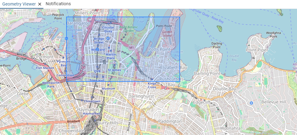
The final query used is to view all geo-data points. Note the geo-data fields are cast as geometry (… ::geometry) here. This is so the data points can be outputted in binary and viewed under the Geometric Viewer in PostgreSQL.
-- 5.4  Visual sanity check — return everything as WKT
SELECT 'Depot'  AS type, name, ST_AsText(loc)  FROM depots
UNION ALL
SELECT 'Zone',  zone_name, ST_AsText(area) FROM delivery_zones
UNION ALL
SELECT 'Cust',  name, ST_AsText(loc)       FROM customers;
Results:
| type | name | st_astext |
|---|---|---|
| Depot | Sydney Depot | POINT(151.207 -33.8675) |
| Zone | CBD Zone | POLYGON((151.1984 -33.86,151.23 -33.86,151.23 -33.875,151.1984 -33.875,151.1984 -33.86)) |
| Cust | Alice Inside | POINT(151.21 -33.865) |
| Cust | Bob Edge | POINT(151.1984 -33.865) |
| Cust | Charlie Outside | POINT(151.25 -33.88) |
This final output when viewed under Geometric Viewer shows all the data points. The original delivery zone here is clearly represented as the blue box hovering around the CBD. The two points within the delivery zone are the depot and sole customer sitting within the zone. The two remaining customers are either residing on the edge or outside the delivery zone.
Wrapping up
Geo‑data isn’t complicated and can be understood in a three‑step flow:
- Store your dots and shapes in proper spatial columns (Geometry – Point, Line, Polygon…”).
- Query them with spatial ST_ functions.
- Visualise the data using graphical maps so it’s clearly understood
In the case study its understood how to determine customers within the delivery radius of a depot and how this looks on an interactive map. Instantly the result was clear on which customers fell in or outside the zone. The takeaway here is any questions requiring geo-data expertise can be easily answered using spatial functions exclusively within SQL.